Adisorn Owatsiriwong, D.Eng.
In real life, the best solution that fulfills a single objective function might not be the best solution for others. It's rare to obtain one solution that beats all objectives. This gives us the motivation to solve multi-objective optimization problems.
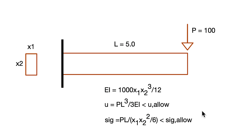
Considering a cantilever beam subjected to loading at the far end, the design objective might be
f1: Minimum deflection
f2: Minimum material volume or weight
The beam design problem is usually subjected to the following constraints
C1: Limit stress at any section to the allowable value
C2: Limit deflection value at the far end
Applying a multi-objective optimization solver, we can get solutions with the multiple values of objective functions, says f1 and f2 plotting below.
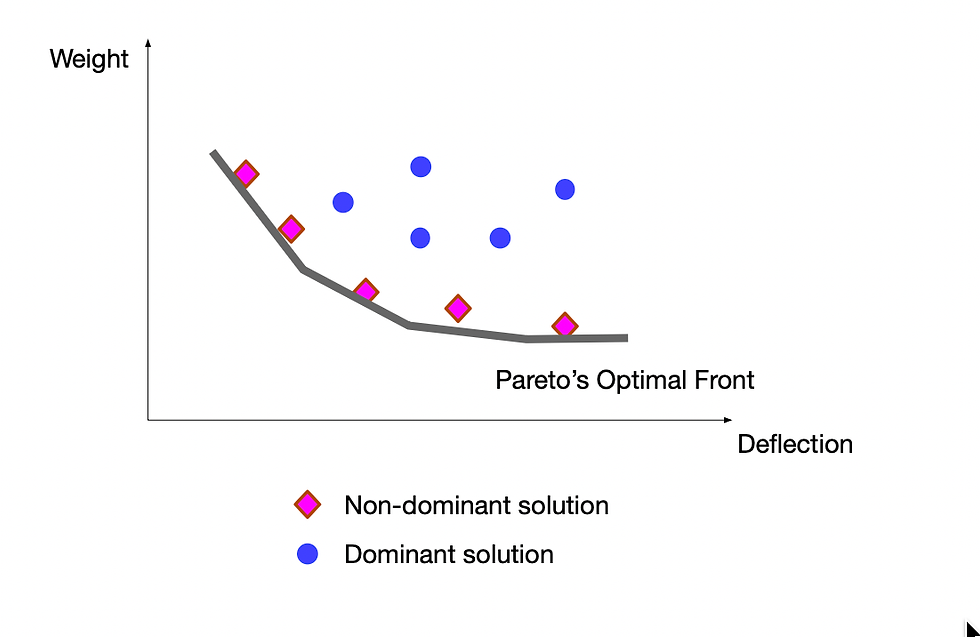
The solutions are classified as dominant (not useful) and non-dominant (useful or Pareto's). We can choose one or any non-dominant solution set as one of our best solutions. The choice of the best solution might be based on the decision maker or other pre-defined criteria.
By definition, for any minimizing problem, x is non-dominant solution if and only if
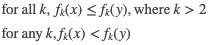
In other words, the solution is non-dominant or Pareto's solution if no objective function can be improved in value without degrading some of the other objective values.
Example:
A cantilever beam has a rectangular section b x h and length L. We are using PSO to obtain the Pareto front for two objectives:
Minimize tip deflection: f1(b,h) = P*L^3/3EI
Minimize material volume: f2(b,h) = b x h x L
To simplify the problem, we make this problem unconstrained. We can always impose the constraints to the problem through the penalty function inside the objective functions.
To achieve this, we have developed a PSO-MOO algorithm to find a set of non-dominated solutions, aka Pareto optimal front in f1 and f2 space.

MATLAB Code:
% Multi Objective Optimimation : Cantilever Beam Example
%
clear all
close all
global L P E
% Problem Definition
numObjectives = 2; % Number of Objectives
numVariables = 2; % Number of Decision Variables [b,h]
varSize = [1, numVariables]; % Size of Decision Variables Matrix
L = 5.0; % Cantilever span length (m)
P = 100; % Tip load kN
E = 2e7; % Elastic Modulus
% PSO Parameters
maxIter = 100; % Maximum Number of Iterations
popSize = 100; % Population Size (Swarm Size)
w = 0.5; % Inertia Weight
wdamp = 0.99; % Inertia Weight Damping Ratio
c1 = 1.5; % Personal Learning Coefficient
c2 = 2.0; % Global Learning Coefficient
lb = [0.2,0.4]; % Lower bound
ub = [0.5,1.0]; % Upper bound
% Initialization
empty_particle.Position = [];
empty_particle.Velocity = [];
empty_particle.Cost = zeros(1, numObjectives);
empty_particle.Best.Position = [];
empty_particle.Best.Cost = zeros(1, numObjectives);
particle = repmat(empty_particle, popSize, 1);
% Initialize Particles
for i=1:popSize
particle(i).Position = lb + rand(varSize).*(ub-lb);
particle(i).Velocity = zeros(varSize);
particle(i).Cost = CostFunction(particle(i).Position);
particle(i).Best.Position = particle(i).Position;
particle(i).Best.Cost = particle(i).Cost;
end
% PSO Main Loop
for it=1:maxIter
for i=1:popSize
% Update Velocity
particle(i).Velocity = w * particle(i).Velocity ...
+ c1 rand(varSize) . (particle(i).Best.Position - particle(i).Position) ...
+ c2 rand(varSize) . (rand(varSize) - particle(i).Position);
% Update Position
particle(i).Position = particle(i).Position + particle(i).Velocity;
if particle(i).Position(1) <= lb(1)
particle(i).Position(1) = lb(1);
end
% check position to be in the boundaries
indx1 = find(particle(i).Position < lb);
indx2 = find(particle(i).Position > ub);
particle(i).Position(indx1) = lb(indx1);
particle(i).Position(indx2) = ub(indx2);
% Evaluation
particle(i).Cost = CostFunction(particle(i).Position);
% Update Personal Best
if Dominates(particle(i).Cost, particle(i).Best.Cost)
particle(i).Best.Position = particle(i).Position;
particle(i).Best.Cost = particle(i).Cost;
end
end
% Damping Inertia Weight
w = w * wdamp;
% Identify Non-Dominated Solutions
paretoFrontIndices = []; % To store indices of particles on the Pareto front
for i = 1:popSize
isNonDominated = true; % Assume this particle is non-dominated
for j = 1:popSize
if i ~= j && Dominates(particle(j).Best.Cost, particle(i).Best.Cost)
isNonDominated = false; % Found a particle that dominates i
break;
end
end
if isNonDominated
paretoFrontIndices = [paretoFrontIndices, i];
end
end
% Correcting the extraction of Pareto Front Costs
paretoFrontCosts = zeros(length(paretoFrontIndices), numObjectives);
paretoFrontPosition = zeros(length(paretoFrontIndices), numVariables);
for i = 1:length(paretoFrontIndices)
paretoFrontCosts(i, :) = particle(paretoFrontIndices(i)).Best.Cost;
paretoFrontPosition(i,:) = particle(paretoFrontIndices(i)).Best.Position;
end
% Plotting the Pareto Front
%figure;
plot(paretoFrontCosts(:,1), paretoFrontCosts(:,2), 'bo');
title('Pareto Front');
xlabel('z-displacement (cm)');
ylabel('Volume (m3)');
grid on;
hold off
end
% Supporting Functions
function z = CostFunction(x)
global L E P
% Example objective functions
b = x(1);
h = x(2);
Iz = b*h^3*1/12;
z1 = P*L^3/3/E/Iz*100;
z2 = L*b*h;
z = [z1, z2]; % Replace with your actual objective functions
end
function b = Dominates(x, y)
% Determines if solution x dominates solution y
b = all(x <= y) && any(x < y);
end

Pareto front at 1st iteration

Pareto front at 100th iteration
It is shown that the PSO-MOO solution has evolved the shape of the Pareto front in f1-f2 space. The Pareto front contains a set of non-dominated solutions (no better solution is improved without worsening another objective function).

One of the favorable solutions can be shown in the figure above (f1,f2 ) = (2.02,0.85), which corresponds to (b,h) = (0.20,0.85).

However, this is unnecessary the best solution when a deflection limit is imposed. For example, consider the maximum deflection L/500 (500/500 = 1 cm). The best solution is then (f1,f2) = (1.0, 1.24), which corresponds to (b,h) = (0.246, 1.00).